3. Tuning details and results

This chapter describes the details and results of the tuning performed according to the procedure in Section 2.2 (Procedure of tuning).

3.1. Evaluation of the performance

To compare with the performance after performing the tuning, the execution time of the Application was measured before performing the tuning. In this tuning work, the Application was divided into measurement regions by reference to the log files that were output by the Application, and the execution time of each measurement region was also measured to make it easier to evaluate the effects of tuning. When discussing the execution time of the Application in this document, both the execution time of the entire Application and the execution time of each measurement region must be described.

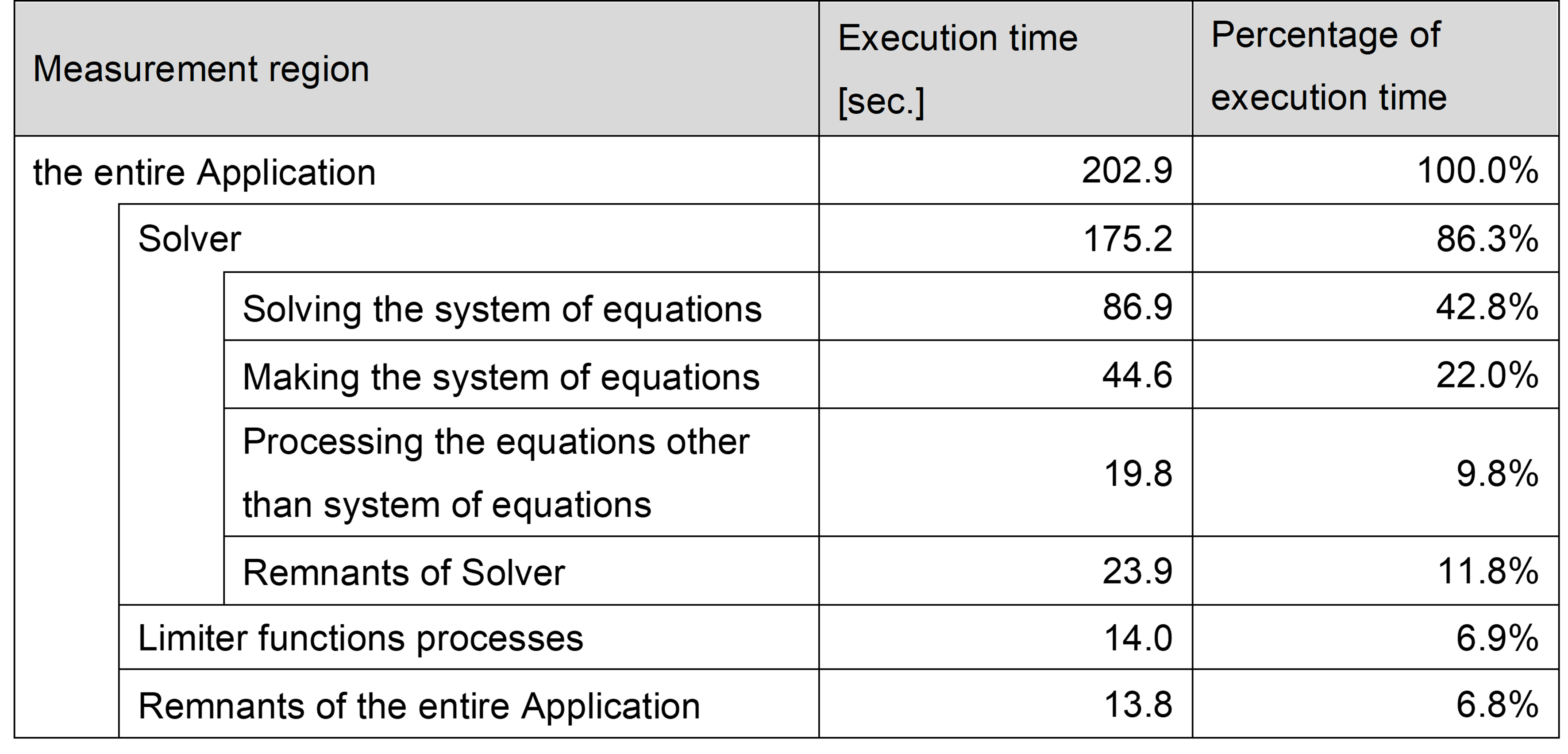
The measurement regions are composed of three portions: “Solver”, “Limiter functions processes”, and “Remnants of the entire Application”. Execution time of “Remnants of the entire Application” is defined as execution time of the entire Application minus execution time of “Solver” and “Limiter functions processes”.

“Solver” was further divided into four portions: “Solving the system of equations”, “Making the system of equations”, “Processing the equations other than system of equations”, and “Remnants of Solver”. Execution time of “Remnants of Solver” is defined as execution time of “Solver” minus execution time of other 3 portions.

The following table shows the execution time of initial version and the execution time of each measurement region. As seen in the table, “Solving the system of equations” is the largest measurement region, and it is 43% of the entire Application.

3.2. Cost of each function

In order to focus on the target functions for tuning, the cost of each function, which is proportional to the execution time of each function, in the initial version was measured by sampling analysis using fipp. As a result, in the initial version with the condition of the tuning, 1645 functions and their costs were output by fipp.

The following table represents the top ten functions by the result of cost information by fipp as samples. Each column in the table represents the following:

• Function: the name of the function

• Measurement region: the name of the measurement region that includes the function in the column “Function”

• Cost: the cost of each function output by fipp

• Percentage of the cost: the percentage of each function’s cost in relation to the total cost of the Application

• Cumulative percentage of the cost: the cumulative percentage of the cost for each function from the first one

	Function	Measurement region	Cost	Percentage of the cost [%]	Cumulative percentage of the cost [%]
0	(the entire Application)	―	10145395	100.00	―
1	calc_function_1	Solving the system of equations	2359630	23.26	23.26
2	function_of_MPI_1	(Related to wait time of an MPI communications)	1818309	17.92	41.18
3	function_of_MPI_2	(Related to wait time of an MPI communications)	1090237	10.75	51.93
4	make_function_1	Making the system of equations	359086	3.54	55.47
5	make_function_2	Making the system of equations	323755	3.19	58.66
6	limiter_function_1	Limiter functions processes	290204	2.86	61.52
7	calc_function_2	Solving the system of equations	187961	1.85	63.37
8	make_function_3	Making the system of equations	176418	1.74	65.11
9	calc_function_3	Solving the system of equation	165032	1.63	66.74
10	make_function_4	Making the system of equations	156562	1.54	68.28

As seen in the table , each cost of the top three functions were larger than 10%, and the sum of their costs is more than 50% of the entire Application.

The function with the highest cost was function “calc_function_1”, which was in the measurement region “Solving the system of equations”, and the percentage of the cost was 23% of the total. The functions “function_of_MPI_1” and “function_of_MPI_2” followed “calc_function_1”. However, they were related to wait time of an MPI communication, hence it was not possible to tune these functions directly.

As seen in the cost of functions other than the top three functions, the percentage of the cost of the fourth function was 3.54% of the total, and the tenth function was only 1.54%. It means that the percentage of the cost of most functions was less than a few percent in the initial version.

3.3. Tuning of the Application

This section describes the tuning items and the Application performance measured after performing the tuning.

3.3.1. Tuning items

The following table represents the tuning details and target functions of all tuning items. Each column in the table represents the following:

• Tuning #: item number for tuning items (Tuning items are assigned numbers in the order in which they were performed.)

• Tuning outline: outline of each tuning item

• Tuning method: the method for performing the tuning, such as specifying OCL(s) (Optimization Control Line) or changing compiler options

• Classification of tuning: classification by reference to the “Programming Guide (Tuning)” that is posted on the user portal site

• Target function: the name of target function of each tuning item

• Measurement region: the name of the measurement region that includes the function in the column “Target function”

• Section #: section number where the details of the tuning item are described

Tuning #	Tuning outline	Tuning method	Classification of tuning	Target function	Measurement region	Section #
1	Loop collapse, and unrolling for loops with small iteration counts	Change the source code	Reduction in the number of instructions	calc_function_1	Solving the system of equations	―
2	Specifying the prefetch instructions	Specify the OCL only	Improved data access waiting by hiding latency	calc_function_1	Solving the system of equations	―
3	Sequential access of addition operations in loops	Change the source code	Improved data access waiting by hiding latency	calc_function_1	Solving the system of equations	―
4	Loop unrolling	Change the source code	Reduction in the number of instructions, and Improved instruction scheduling with loop optimization	calc_function_1	Solving the system of equations	―
5	Loop unrolling	Change the source code	Reduction in the number of instructions, and Improved instruction scheduling with loop optimization	calc_function_1	Solving the system of equations	―
6	Suppressing the faddv instructions	Add extra compile options	Reduction in the number of instructions	calc_function_1	Solving the system of equations	―
7	Loop unrolling	Specify the OCL only	Reduction in the number of instructions, and Improved instruction scheduling with loop optimization	make_function_2	Making the system of equations	―
				make_function_3	Making the system of equations
8	Reordering off-diagonal elements in matrixes	Change the source code	Sequential access	calc_function_1	Solving the system of equations	―
9	Suppression of SIMDization for loops with small iteration counts	Specify the OCL only	Reduction in the number of instructions	calc_function_3	Solving the system of equations	―
				make_function_1	Making the system of equations
				make_function_4	Making the system of equations
				make_function_5	Making the system of equations
				make_function_6	Making the system of equations
10	SIMDization of division operations and suppression of SIMDization for loops with small iteration counts	Change the source code	Improved operation wait for facilitation of SIMDization	calc_function_3	Solving the system of equations	Section 4.1
11	Reducing load and store operations of data by loop unrolling	Change the source code	Reduction in the number of instructions, and Improved instruction scheduling with loop optimization	calc_function_1	Solving the system of equations	Section 4.2
12	Loop unswitching	Specify the OCL only	Improved data access waiting by hiding latency	make_function_5	Making the system of equations	―
13	Loop unrolling	Specify the OCL only	Reduction in the number of instructions, and Improved instruction scheduling with loop optimization	make_function_2	Making the system of equations	―
14	Changing the parameters of domain decomposition of input models	Change settings at execution	Improved the load balance between MPI processes	―	―	―
15	Removing extra type conversion instructions	Change the source code	Reduction in the number of instructions	make_function_2	Making the system of equations	―
16	SIMDization by loop collapse	Change the source code	Improved operation wait for facilitation of SIMDization	make_function_6	Making the system of equations	Section 4.3
17	SIMDization by loop fission	Change the source code	Improved operation wait for facilitation of SIMDization	make_function_2	Making the system of equations	―
18	Inline expansion	Change the source code	Reduction in the number of instructions	limiter_function_1	Limiter functions processes	―
				make_function_1	Making the system of equations
				make_function_4	Making the system of equations
				make_function_9	Making the system of equations
				calc_function_2	Solving the system of equations
				calc_function_3	Solving the system of equations
				calc_function_5	Solving the system of equations
19	Changing the access direction of arrays	Change the source code	Improved data access waiting by hiding latency	othSolv_function_3	Processing the equations other than system of equations	Section 4.4
20	Movement of invariant expressions	Change the source code	Improve waiting for operations by hiding latency	make_function_8	Making the system of equations	―
21	Loop fission	Change the source code	Reduction in the number of instructions, and Improved instruction scheduling with loop optimization	make_function_8	Making the system of equations	―
22	Allocating some arrays in loops to register	Change the source code	Improved data access waiting by hiding latency	make_function_8	Making the system of equations	―
23	Reducing the extra cost in calculation operations	Change the source code	Reduction in the number of instructions	make_function_8	Making the system of equations	―
24	SIMDization by SVE ACLE	Change the source code	Improved operation wait for facilitation of SIMDization	calc_function_4	Solving the system of equations	Section 4.5
25	Built-in prefetch	Change the source code	Improved data access waiting by hiding latency	make_function_2	Making the system of equations	Section 4.6
				make_function_3	Making the system of equations
				make_function_7	Making the system of equations
26	Allocating some arrays to static arrays for SIMDization	Change the source code	Improved operation wait for facilitation of SIMDization	calc_function_1	Solving the system of equations	―
27	Using CLONE specifier, and loop unrolling	Change the source code	Improved data access waiting by hiding latency	make_function_6	Making the system of equations	―
				make_function_12	Making the system of equations
28	Moving division operations to outside of the loop, and applying SIMDization to the division operations	Change the source code	Improved operation wait for facilitation of SIMDization	make_function_7	Making the system of equations	Section 4.7
29	Built-in prefetch	Change the source code	Improved data access waiting by hiding latency	othSolv_function_1	Processing the equations other than system of equations	―
				othSolv_function_2	Processing the equations other than system of equations
				othSolv_function_5	Processing the equations other than system of equations
30	SIMDization by inline expansion	Change the source code	Improved operation wait for facilitation of SIMDization	function_1	Processing the equations other than system of equations	―
				function_2	Processing the equations other than system of equations
31	Thread parallelization	Change the source code	Thread parallelization	calc_function_1	Solving the system of equations	―
				make_function_7	Making the system of equations
32	Improving load instructions scheduling	Change the source code	Improved instruction scheduling with loop optimization	othSolv_function_4	Processing the equations other	―
33	Moving invariant expressions to outside of the loop	Change the source code	Improved instruction scheduling with loop optimization	calc_function_2	Solving the system of equations	Section 4.8
34	Loop unrolling manually instead of OCLs	Change the source code	Reduction in the number of instructions, and Improved instruction scheduling with loop optimization	calc_function_4	Solving the system of equations	Section 4.9
35	Allocating some arrays in loops to register	Change the source code	Improved data access waiting by hiding latency	calc_function_4	Solving the system of equations	―
				calc_function_5	Solving the system of equations
36	Loop interleaving	Change the source code	Improve waiting for operations by hiding latency	calc_function_1	Solving the system of equations	―
37	Removing extra type conversion instruction	Change the source code	Reduction in the number of instructions	calc_function_1	Solving the system of equations	―
38	Specifying the prefetch instructions	Change the source code	Improved data access waiting by hiding latency	calc_function_1	Solving the system of equations	―
39	Loop collapse	Change the source code	Improved instruction scheduling with loop optimization	make_function_6	Making the system of equations	―
				make_function_5	Making the system of equations
40	Using CLONE specifier, and inline expansion	Change the source code	Reduction in the number of instructions, and Improved instruction scheduling with loop optimization	make_function_6	Making the system of equations	―
				make_function_5	Making the system of equations
				make_function_7	Making the system of equations
41	Improving the memory placement of two-dimensional arrays for sequential access	Change the source code	Sequential access	allocate_array	(the entire Application)	Section 4.10
				clear_array	(the entire Application)
				deallocate_array	(the entire Application)
				reallocate_array	(the entire Application)
				allocate_array_2	(the entire Application)
				deallocate_array_2	(the entire Application)
				reallocate_array_2	(the entire Application)
42	SIMDization based on the Tuning #41	Change the source code	Improved operation wait for facilitation of SIMDization	calc_function_1	Solving the system of equations	―
43	Using CLONE specifier	Change the source code	Improved instruction scheduling with loop optimization	make_function_7	Making the system of equations	―
44	Suppression of SIMDization for loops which has built-in prefetch functions	Specify the OCL only	Reduction in the number of instructions	make_function_7	Making the system of equations	―

This document describes ten of forty-four tuning items as samples in Chapter 4 (Tuning items). The details of these ten tuning items are as follows:

• The tuning with local code changes

  These are tuning items that improve performance without significant changes to the source code, such as specifying the OCL(s) in Section 4.2.

  • Section 4.1: SIMDization of division operations and suppression of SIMDization for loops with small iteration counts

  • Section 4.2: Reducing load and store operations of data by loop unrolling

  • Section 4.3: SIMDization by loop collapse

  • Section 4.4: Changing the access direction of arrays

  • Section 4.7: Moving division operations to outside of the loop, and applying SIMDization to the division operations

  • Section 4.8: Moving invariant expressions to outside of the loop

  • Section 4.9: Loop unrolling manually instead of OCLs

• Advanced tuning for improving the performance of the A64FX processor

  These are tuning items that take advantage of the characteristics of the A64FX processor to improve performance, such as using SVE ACLE, specific to Arm, in Section 4.5.

  • Section 4.5: SIMDization by SVE ACLE

  • Section 4.6: Built-in prefetch

• Tuning to the functions which are called from many other functions

  The targets of tuning, described in Section 4.10, are some functions that allocate or deallocate memory for two-dimensional arrays. While the cost of each function was low, these were called by many other functions. Therefore, tuning these functions was expected to improve the performance of the entire Application.

  • Section 4.10: Improving the memory placement of two-dimensional arrays for sequential access

3.3.2. Tuning results

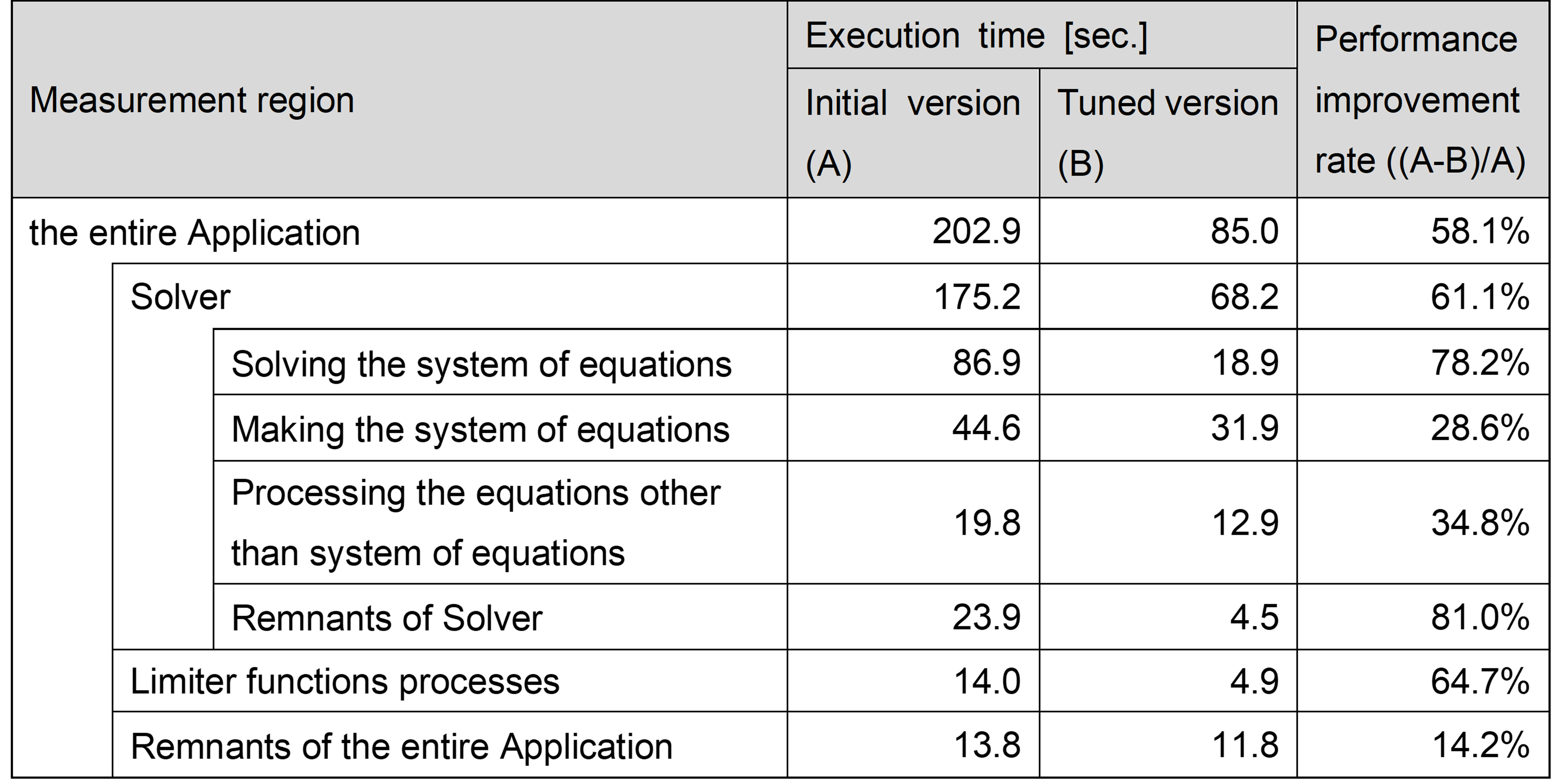
The following table represents the execution time of the initial version and the tuned version (performed tuning items of #1 to #44), and the performance improvement rate comparison between the initial version and the tuned version. As seen in the table, the performance improvement rate of the entire Application is 58%, in other words, the execution time of the tuned version was less than half of the initial version, thus the target performance was achieved.

In this tuning work, the performance of the Application was measured 13 times in the process of performing the 44 tuning items, and the following each graph (Figure 1 or Figure 2) shows these results. In Figure 1, the horizontal axis represents the n-th tuning item as listed in the table in Section 3.3.1 (Tuning items), and the vertical one represents the execution time of the Application measured just after the n-th tuning. Note that height of the vertical bar and the number at the top indicate the execution time of the entire Application. In Figure 2, the horizontal axis represents the same as Figure 1, and the vertical one represents the performance improvement rate, comparing the initial version and after performing the n-th tuning.

For example, the number “8”on the horizontal axis indicates that the Application measured just after the 8th tuning item as listed in the table in Section 3.3.1 (Tuning items). Hence, the data at the vertical axis “8” in Figure 1 shows the execution time of the Application after performing the tuning items #1 to #8. Note that the data at the position of the horizontal axis 0 shows the data of initial version.

Figure 1: The execution time of the entire Application measured just after performing the n-th tuning.

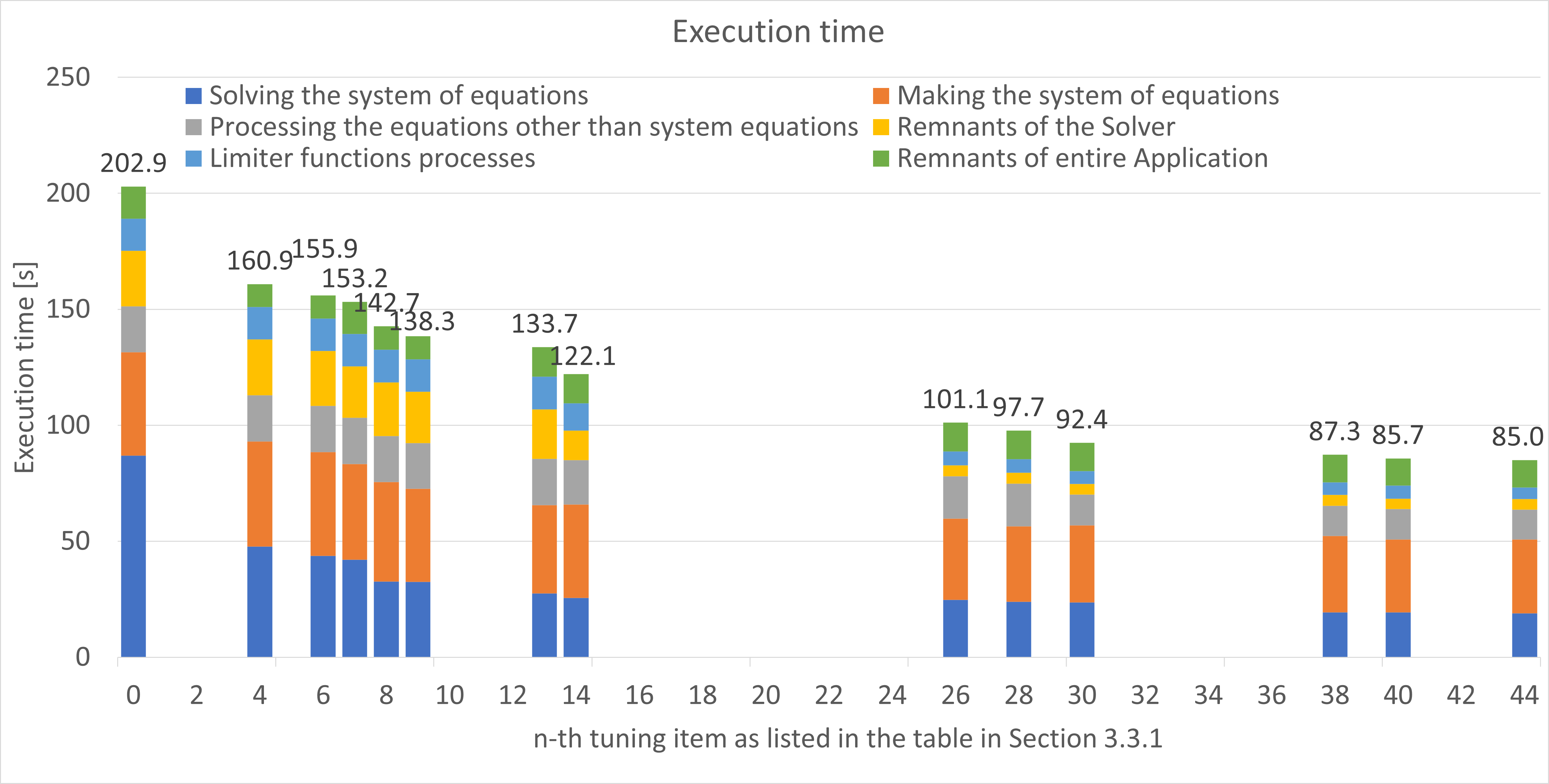
Figure 2: The performance improvement rate, comparing the initial version and after performing the n-th tuning.

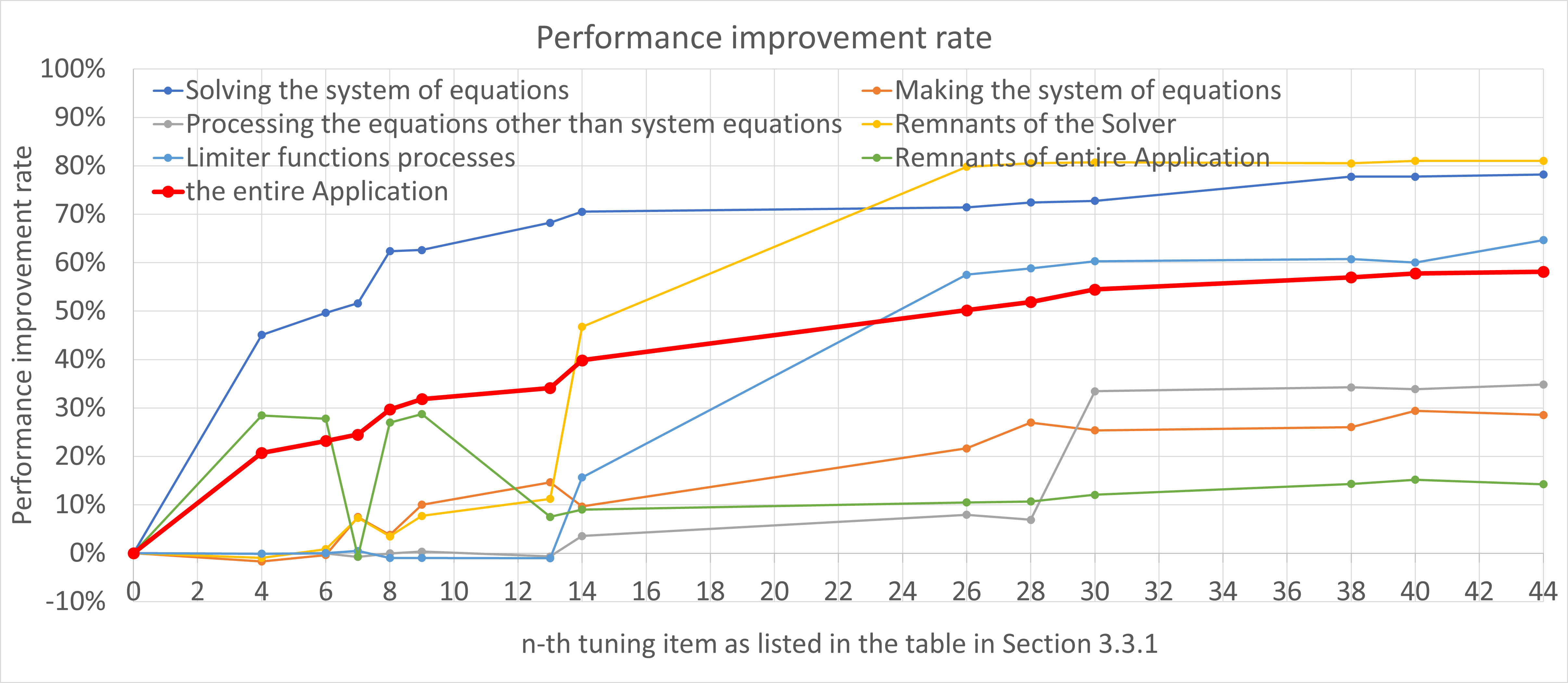
As seen in the Figure 2, the entire Application was improved by about 34% and the performance of the “Solving the system of equations“ was improved by about 68% from the 1st to the 13th tuning item. The first 13 tuning items were targeted for the top eight highest cost functions, and especially 7 of them were targeted for the function “calc_function_1”, which was the function with highest cost in the initial version.

In Figure 2, the graph shows a steep increase of “the entire Application” (about 34% to 40%) from the 13th to the 14th tuning item. The 14th tuning item improved the load imbalance between processes by changing execution parameters of the domain decomposition of the Application, and it was performed according to the suggestion given by the ISV who developed the Application.

Additionally, the performance of the entire Application further improved by about 18% by performing the 15th to the 44th tuning item, which was targeted for lower-cost (other than the top three functions in the table in Section 3.2) functions. Therefore, each performance improvement rate of the tuning item to the entire Application was smaller than those of the 1st to the 14th tuning item.

Focusing on the performance improvement rate for each measurement region in Figure 2, tuning items #1 to #13 contribute significantly to the performance improvement of “Solving the system of equations”. Similarly, #14 contributes to “Remnants of Solver”, #15 to #26 contribute to “Limiter functions processes”, and #28 to #30 contribute to “Processing the equations other than system of equations”.

In summary, 44 tuning items were performed, which led to the reduction of the execution time of the entire Application from 202.9 seconds to 85.0 seconds (about 2.4 times faster) and the achievement of the target performance (reduction of the execution time to less than half). The details are as follows:

• 40 items were targeted for the top 30 functions that account for about 52% (except functions related to the MPI communications) of the entire Application.

• 2 items were targeted for the low-cost functions that were called from various parts of this Application (one of which was described in Section 4.10 (Improving the memory placement of two-dimensional arrays for sequential access)).

• 1 item: improvement of load balance between processes

• 1 item: implementation of thread parallelization

Column: For large-scale simulations at Fugaku

The tuning items #14 and #31 are especially important to execute the large-scale simulations using hundreds of thousands of CPU cores, which are required by users.

#14: Changing the parameters of domain decomposition of input models

In this tuning item, the parameters of decomposition were changed to improve the load balance between MPI processes. Improving the load balance between MPI processes leads to reduce the communication latency between MPI processes. Also, the impact on the latency will be getting larger as the number of processes increases. Therefore, it is important to balance the amount of operations performed by each process.

#31: Thread parallelization

The initial version of the Application did not support thread parallelization. However, thread parallelism is crucial for executing the large-scale simulations using hundreds of thousands of CPU cores more efficiently. Therefore, thread parallelization was performed. This is the first time that thread parallelization has been performed on the Application. In this tuning item, thread parallelization was performed only for the functions “cal_function_1” and “make_function_7”, which do not include factors inhibiting thread parallelization such as data conflicts, were therefore easy to implement. The percentage of the cost of the two functions accounted for about 25% in the initial version.

The execution conditions, such as the model and parallel number, in this tuning work are not large enough to evaluate the performance of large-scale simulations using hundreds of thousands of CPU cores. Therefore, after the 44 tuning items were performed, a simulation of the larger-scale model with about 800 million elements was carried out on Fugaku to evaluate the effect of the tuning. The simulation was executed using over 4000 compute nodes, with hybrid MPI-OpenMP parallelism (with 4 threads). As a result, it completed with up to about 220,000 CPU cores, and also the speed-up was observed up to about 200,000 CPU cores. The execution of the much larger-scale simulations is expected by further improvements, such as thread parallelization of the other loops.